Importing With Record IDs Using Excel's VLOOKUP
Overview
Sugar®'s import wizard allows users to easily update existing records by referencing each records' unique ID number. For more information about updating records via import, see the Knowledge Base article Updating Records via Import. There may be occasions, though, when the update file does not contain the ID field for the records you want to update. In these situations, you can use the Microsoft Excel® VLOOKUP function to insert the correct ID for each row of your spreadsheet.
Understanding Excel's VLOOKUP
The VLOOKUP function allows you to connect two sets of data using a common field value. For example, a spreadsheet containing only names and email addresses can be joined with a spreadsheet containing only names and phone numbers by virtue of the common name field. 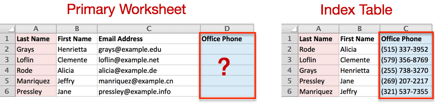
In the example above, the primary worksheet holds the email address for Ms. Grays, and the index table holds the phone number for Ms. Grays. As long as the Last Name column exists on both sheets, it is possible to make Excel communicate information from one sheet to the other. To bring the missing phone number value into the primary worksheet, we will add column D titled "Office Phone", and in that column, reference the index table. Before delving into the details for doing this, here is an in-depth look at how a VLOOKUP works.
Mastering the VLOOKUP Formula Elements
The "V" in VLOOKUP stands for "vertical". It refers to the vertical column of data values that will be used to connect to your primary workbook and return a field value from the corresponding row. The Excel formula for a VLOOKUP is:
=VLOOKUP(lookup_value,table_array,col_index_num,[range_lookup])
| Excel Formula Element | Description |
|
lookup_value |
This is the unique value from the primary worksheet that you will match to a unique value in a separate index table. In the example tables above, the lookup value will be in column A for each row of the primary worksheet. Column A contains the common data between the two sheets, which is also the data that you want Excel to search for in the index table.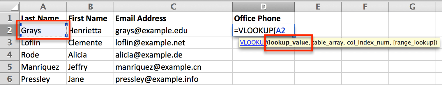 |
| table_array |
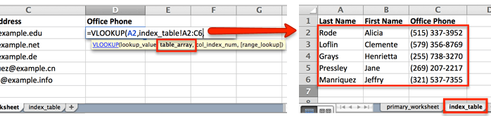
The table array is a range of cells that make up your index table. This array can be part of the active worksheet, on a different worksheet, or even in a different file. The table array must have a column containing the values that correspond with the lookup value, and that column must be the first column in the table. In this example, the table array is on the index table worksheet and starts with cell A2 (do not include header rows) and extends to cell C6.
|
| col_index_num |
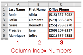
Because the index table may be more than two columns wide, and the first column always contains the lookup values, the return column index number tells Excel which column number's values you want to pull into the primary worksheet. This is expressed as an integer and is relative to the first column of data in the index table (e.g., when the table spans columns A-C, column A contains the lookup values and is column index number 1, column B is column index number 2 and column C is column index number 3). In the example above, we would like to return the phone number values from column C, therefore the return column index number is 3. |
| range_lookup | This boolean (true/false) value represents whether the lookup value requires an exact character match from the index table or if Excel should find an approximate match. When set to "TRUE", Excel will consider the most similar value a match when an exact match is not found. For most Sugar import functions we will set this to "FALSE" in order to require an exact character match. |
The Excel formula for the first row of data for the example tables above will look like this:
=VLOOKUP(A2,index_table!A2:C6,3,FALSE)
Using Absolute References in Excel Formulas
Once you have crafted the formula for the first row of the import file, the next step is to copy this formula to the following rows. As illustrated by the following sample data, when you copy a formula from one row to the next, the formula will automatically update cell references relative to the position of the row.
|
A |
B |
|
| 1 | id | |
| 2 | aaa@gmail.com | =VLOOKUP(A2,index_table!A2:C6,3,FALSE) |
| 3 | bbb@gmail.com | =VLOOKUP(A3,index_table!A3:C7,3,FALSE) |
| 4 | ccc@gmail.com | =VLOOKUP(A4,index_table!A4:C8,3,FALSE) |
| 5 | ddd@gmail.com | =VLOOKUP(A5,index_table!A5:C9,3,FALSE) |
In this example, the red lookup value must adjust incrementally in order for the VLOOKUP formula to reference the respective email address for each row. The blue values in the table range, however, also adjust automatically. This is not desired behavior because the table_array range will remain static regardless of the formula's row position. In this example, the table range location will always be index_table!A2:C6. In order to lock the range in place and avoid Excel's auto-increment feature, use Excel's absolute cell reference indicator $ before each row and column value that should remain static.
For example, the earlier formula =VLOOKUP(A2,index_table!A2:C6,3,FALSE) will become =VLOOKUP(A2,index_table!A2:$C$6,3,FALSE) after adding the necessary $ absolute cell reference indicators.
Note: References to a table array in a separate file will automatically use absolute references and do not need to be edited. References to a table array located in the active file – even if in a separate worksheet – must be edited for absolute table array references.
Application
Use Case
For the following steps, we have acquired a list of names and email addresses from visitors to our booth at a biotechnology tradeshow. The names on the list may or may not be in Sugar already. If the person is not a contact in Sugar, we will need to import that person as a new contact. If the person is already a contact in Sugar, the existing contact record should be updated with the new data. Follow these steps to find out if the new list contains any existing contacts and if so, extract those contacts' Sugar IDs via each record's email address.
Steps to Complete
Step 1 : Creating a Sugar Report to Use as an Index Table
Export a list of contacts and their IDs from a Sugar report to use as the index table for comparison with the tradeshow list.
- Create a new "Rows and Columns Report" for Contacts. For detailed steps to create a rows and columns report, refer to the Reports documentation.
- Define the following filters:
- Contacts > Account > Industry > Is > Biotechnology
- Contacts > Email Address > Email Address > Is Not Empty
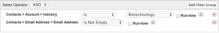
- Choose the display columns in the following order:
- Contacts > Email Addresses > Email Address
- Contacts > ID
- Contacts > First Name
- Contacts > Last Name

- Name the report "Biotechnology ID Index".
- Click "Save & Run" to see the results and then click "Export" from the report's actions menu.
Step 2 : Assembling the VLOOKUP formula
In Excel, open both the exported file Reports.csv from your downloads folder and the tradeshow list that you plan to import. Make the following adjustments to the tradeshow import file:
- Insert a column at the beginning of the spreadsheet (column A). In the header row of the new column A, type the label "Contact ID".
- In cell A2, craft a VLOOKUP formula. Type
=VLOOKUP(. - Click the cell in row 2 that contains an email address. This will automatically insert the cell reference into the formula.
- Type
,(comma).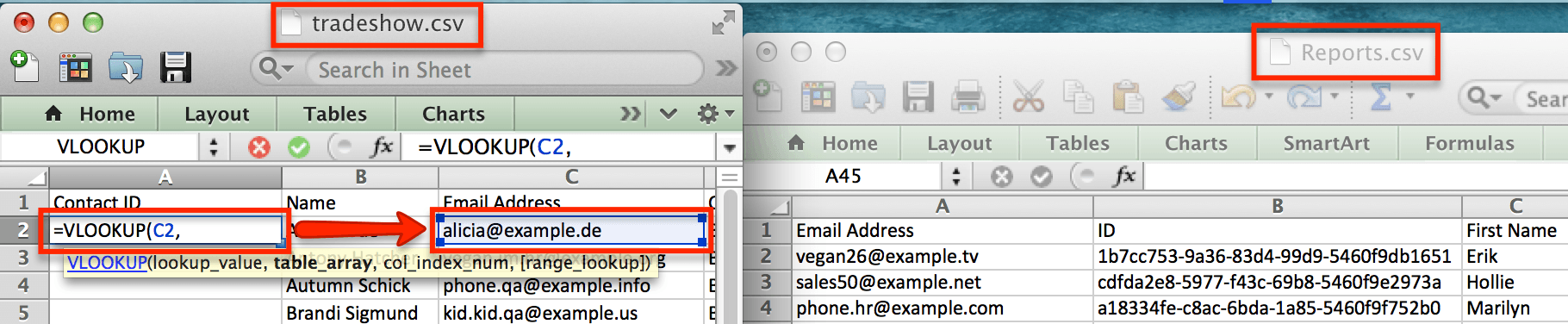
- Click on the window of the Reports.csv file to bring it forward. For the Table Array formula value, click on cell A2 of this sheet and, while holding down the shift key, click the cell that represents the last row and column of the exported data. In the example below, the end of the array table is cell D20.
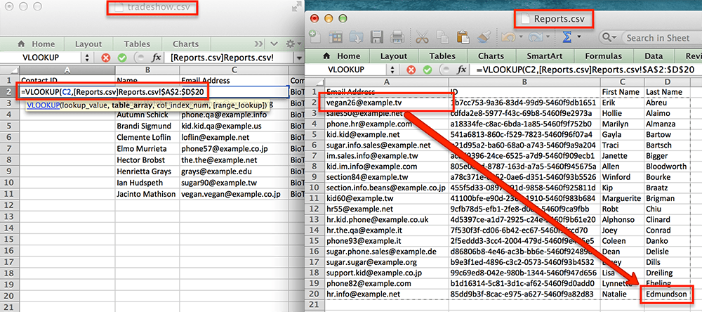
The VLOOKUP formula is now halfway complete and will look similar to this: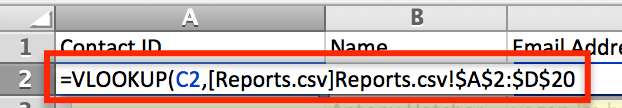
Note: This table array references a separate file and will therefore automatically use absolute references. - Type another
,(comma). - Type the column number associated with the ID data in the Reports.csv table array. In this example, the ID is in the 2nd column so we will enter the number
2. - Type another
,(comma). - Type the word FALSE for exact matches and close the formula's parentheses:
FALSE). The VLOOKUP formula is now complete and should look similar to this: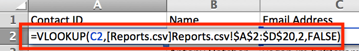
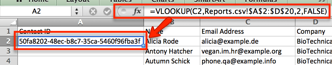
- Press enter on the keyboard. The formula will tell Excel to search the Reports.csv file for a matching email address and, if found, display the ID value from the adjacent column.
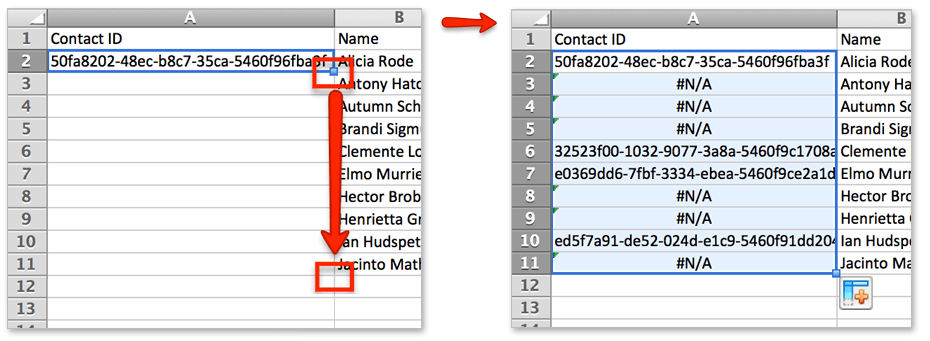
- Pull the formula down to the remaining column cells by clicking and holding the tiny square in in the corner of the selected cell and pulling straight down. Any rows that do not have a corresponding Sugar record will display "#N/A" to indicate that no exact email match was found. Rows that display a valid contact ID are representative of contacts that already exist in Sugar.
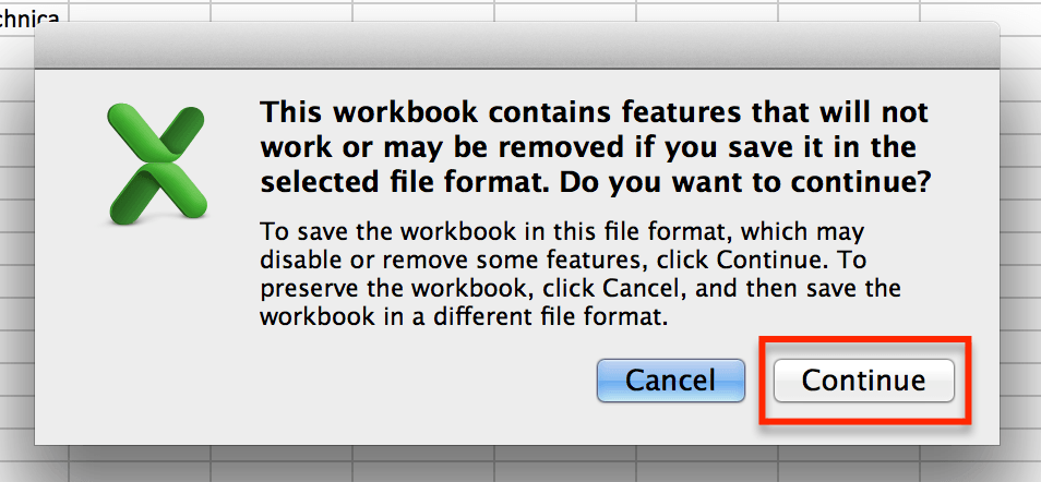
- Save this amended tradeshow list as a CSV file. On save, Excel will display a warning that CSV file formats have less robust feature support than XLS or XLSX files. This is ok. Click Continue to save the file.
Step 3 : Preparing the Import File
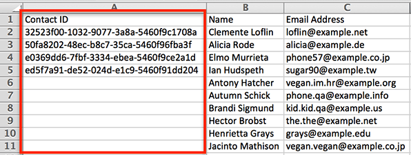
Re-open the tradeshow import CSV file saved in the previous step. Notice that the Contact ID column has now converted from formulas to their calculated values. Prepare this file for import.
- Sort the data by Contact ID and clear the contents of all cells that contain "#N/A". These rows will be created as new contacts in Sugar.
- If desired, separate first names and last names into separate columns. Note that the VLOOKUP function can do this for known Sugar contacts by adapting the steps above to retrieve the First Name and Last Name columns from Reports.csv.
- Arrange the remaining data as appropriate according to the Introduction to Importing article.
Step 4 : Importing the New and Existing Contacts to Sugar
Finally, perform the import in Sugar. From the Contacts module tab, select "Import Contacts".
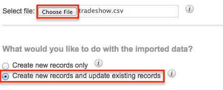
- For step 1 of the import wizard, choose "A file on my computer". Click "Next".
- For step 2 of the import wizard, select the CSV file that contains the tradeshow names and available contact IDs, and then select "Create new records and update existing records". This will ensure that duplicate contacts are not created during the import. Instead, existing contacts will be updated with the most recent data found in the import file.
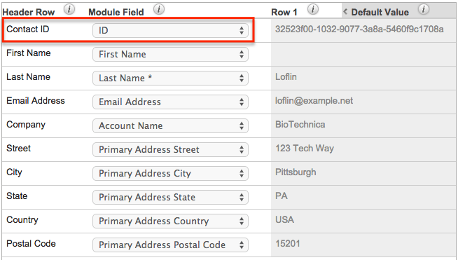
- Complete the import wizard as instructed in the Knowledge Base article, Updating Records via Import. Be sure to map the incoming header row values to the appropriate Sugar fields. For example, the header row "Contact ID" must be mapped to the Sugar Contacts module field "ID".
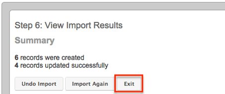
- After the import is complete, the View Import Results summary will display the total number of created contacts and the total number of updated contacts. Check the results carefully for any errors and then click "Exit" to complete the import process.